使用tensorflow實作word2vec CBOW

最近在上udacity的deep learning課程，花了一些時間研究word2vec及skip-gram/CBOW在幹嘛，決定趁熱筆記一下

什麼是word2vec?

如字面意義就是word to vector，也就是將一個字(或詞)轉成向量(也稱為embedding)，將字投到一個多維的空間，相較於傳統的bag of words作法(也就是每個column對應一個單字)，word2vec更能看出字與字間的關係，在該多維空間中越接近的向量通常越相似，而因為每個維度表示某種意義，空間中的方向也往往表示字與字間的某種關係。

在向量化後就能做些有趣的向量操作，最經典的例子是king – man + woman = queen

如何做word2vec?

word2vec是一種打假球(?)的做法，使用資料訓練一個兩層的neural network，讓他預測會出現的字(依據輸入與輸出資料的關係分成CBOW及skip-gram兩種)，但訓練完後不使用這個neural network，只使用embedding的部分。

背後的理論為相似的字周圍的字通常會比較相似，而我們訓練出來的neural network為了要讓相似的輸入(字)有相似的輸出，在embedding這層使用的權重就會趨於一致

CBOW與Skip-Gram的差異

**下面兩張圖片來自這裡**

fig-word2vec-cbow fig-word2vec-sg

左: CBOW，右: skip-gram，圖中的W矩陣就是最後會拿來用的embeddings，W的每個row就是每個字對應的向量(embedding)

例句: neural item embedding for collaborative filtering

CBOW(continuous bag of words)

使用周圍的字預測中間的字，以上面的例句為例，我們希望輸入輸出像下面這樣(假設window_size=1，也就是只拿前後各一個字):

輸入: (neural, embedding)，輸出: item

在實作時跟上面圖片有點差異是會把所有輸入的字的embedding做平均再丟進W’得到最後的輸出，而也因為這個平均的動作，在資料量不夠大的時候CBOW的表現會比skip-gram好(我想大概是因為比較不容易overfitting)

Skip-Gram

使用中間的字預測周圍的字，以上面例句為例，我們希望輸入為"item"時，輸出會是"neural"跟"embedding"，不過跟上面圖不一樣的是，實際上餵給neural network的資料會是兩組: (item, neural)跟(item, embedding)，而不是輸入"item"輸出直接是"neural"跟"embedding"兩個字

從兩者的實作也可以看出來，在window裡面字的先後順序是沒有影響的

講這麼多終於要開始實作了，skip-gram的部分是直接使用udacity提供的code，有興趣的人可以從這裡下載ipython notebook(其實當初花最多時間的是在看裡面的generate_batch在幹嘛)，而這篇文章對應的code放在我的github上

共同參數:

batch_size: 每一回合要丟多少training example進去train
embedding_size: 最後做出來的字向量(vector)有多少維度(dimension)
window_size: 要考慮前後幾個字(當window_size=1時考慮左右各一個字)
num_sampled: 為了增加training的效率，word2vec在做back propagation時只會更新送進去的training labels以及隨機取的num_sampled個negative sample(也就是預測結果應該為0的幾個字)對應的參數(word2vec在back prop的實作上有兩種hierarchical softmax跟negative sampling，這邊用的是後者)而不識像一般的neural networks更新所有的neuron
vocabulary_size: 只考慮最常出現的n個字，在把文章轉矩陣的過程中若是在此n個字以外的字就會被丟棄，因此也不會出現在word2vec的結果裡(在實作中他們全會被轉成’UNK’這個字)

graph的定義:

分成兩個部分: 變數以及operation，因為兩個很像這邊以cbow作範例


self.train_dataset = tf.placeholder(tf.int32, shape=[self.batch_size, 2*self.window_size])
 self.train_labels = tf.placeholder(tf.int32, shape=[self.batch_size, 1])

# Variables.
 embeddings = tf.Variable(tf.random_uniform([self.vocabulary_size, self.embedding_size], -1.0, 1.0))
 softmax_weights = tf.Variable(tf.truncated_normal([self.vocabulary_size, self.embedding_size],
 stddev=1.0 / math.sqrt(self.embedding_size)))
 softmax_biases = tf.Variable(tf.zeros([self.vocabulary_size]))

# Model.
 # Look up embeddings for inputs.
 embed = tf.reduce_mean(tf.nn.embedding_lookup(embeddings, self.train_dataset), axis=1)
 # Compute the softmax loss, using a sample of the negative labels each time.
 self.loss = tf.reduce_mean(tf.nn.sampled_softmax_loss(weights=softmax_weights,
 biases=softmax_biases, inputs=embed, labels=self.train_labels, num_sampled=self.num_sampled,
 num_classes=self.vocabulary_size))

# Optimizer.
 # Note: The optimizer will optimize the softmax_weights AND the embeddings.
 # This is because the embeddings are defined as a variable quantity and the
 # optimizer's `minimize` method will by default modify all variable quantities
 # that contribute to the tensor it is passed.
 # See docs on `tf.train.Optimizer.minimize()` for more details.
 self.optimizer = tf.train.AdagradOptimizer(1.0).minimize(self.loss)

# Compute the similarity between minibatch examples and all embeddings.
 # We use the cosine distance:
 norm = tf.sqrt(tf.reduce_sum(tf.square(embeddings), 1, keep_dims=True))
 self.normalized_embeddings = embeddings / norm

變數:

train_dataset: 這一回合的training input，因為每一回合送進去的東西都不同，所以使用tf.placeholder而不是tf.Variable，在session裡面再透過feed_dict把資料送進去
train_labels: 這一回合的training output，跟train_dataset一樣是tf.placeholder
embeddings: 最後會實際被拿來使用的部分(也就是上面圖中左邊的部分W)，每個row就是一個word vector
softmax_weights & soft_max_biase: 相當於上面圖中的W’，經過處理的結果會再算softmax以取得最後輸出的每個字的機率
normalized_embeddings: 最後model會輸出的word2vec的結果，是把embeddings normalized後的矩陣

operation

tf.nn.embedding_lookup: tensorflow內建的方法，使用這個就不用先把input做one-hot encoding就可以拿到每個input對應的embedding (像前面說過的CBOW會取平均，所以前面多加tf.reduce_mean)
tf.nn.sampled_softmax_loss: 搭配上面講的negative sampling，tensorflow裡內建的方法可以幫我們直接把negative sampling下的softmax loss算出來

Skip-gram

獨有的參數為num_skips，就是同一個字要產生幾組training data也就是要抓window裡的幾個字出來，這也是為什麼一開始會assert num_skips <= 2 * window_size，因為windown裡就只有widow_size *2這麼多個字。

以上面的例句"neural item embedding for collaborative filtering"為範例，若num_skips為2，則對於"item"這個target會產生2組training_data: (embedding ,xxx)與(embedding,yyy )，實際上xxx跟yyy會是什麼則要看實際上window_size抓多大以及在產生batch data時到底隨機取了哪些字。若window_size = 2, skip_size = 3，則最後產生batch時就會在以下幾種組合裡取3個: (embedding, neural), (embedding,item), (embedding, for), (embedding, collaborative)

而這個參數也會影響在每次產生batch時label究竟會看幾個字，如果batch_size為128，而num_skips為4，則每次batch裡面會有的獨特的label的字的數量就是128/4 = 32

generate_batch


batch = np.ndarray(shape=(self.batch_size), dtype=np.int32)
 labels = np.ndarray(shape=(self.batch_size, 1), dtype=np.int32)
 span = 2 * self.window_size + 1 # [ window_size target window_size ]
 buffer = collections.deque(maxlen=span)
   for _ in range(span):
     buffer.append(data[self.data_index])
     self.data_index = (self.data_index + 1) % len(data)
 for i in range(self.batch_size // self.num_skips):
     target = self.window_size # target label at the center of the buffer
     targets_to_avoid = [self.window_size]
     for j in range(self.num_skips):
       while target in targets_to_avoid:
         target = random.randint(0, span - 1)
         targets_to_avoid.append(target)
         batch[i * self.num_skips + j] = buffer[self.window_size]
         labels[i * self.num_skips + j, 0] = buffer[target]
     buffer.append(data[self.data_index])
     self.data_index = (self.data_index + 1) % len(data)
 return batch, labels

CBOW

使用周圍的字預測中間的字，所以我自己在做的時候把前後不足window_size的字都跳過，以上面的例句"neural item embedding for collaborative filtering"而言，若window_size = 2，則item和neural都不會做為target，也就是這個句子產生的第一組資料為((“neural","item","for","collaborative"), “embedding")，最後一組為((“item","embedding","collaborative","filtering"), “for")

generate batch


batch = np.ndarray(shape=(self.batch_size, 2*self.window_size), dtype=np.int32)
 labels = np.ndarray(shape=(self.batch_size, 1), dtype=np.int32)

for i in range(self.batch_size):
 # skip head and tail
 while self.data_index - self.window_size &lt; 0:
   self.data_index += 1
 if (self.data_index + self.window_size) > len(data):
   # start all over again
   self.data_index = self.window_size
 for j in range(self.window_size):
   batch[i, j] = data[self.data_index - self.window_size + j]
   batch[i, j + self.window_size] = data[self.data_index + (j + 1)]
   labels[i, 0] = data[self.data_index]
   self.data_index += 1
 return batch, labels

結果比較

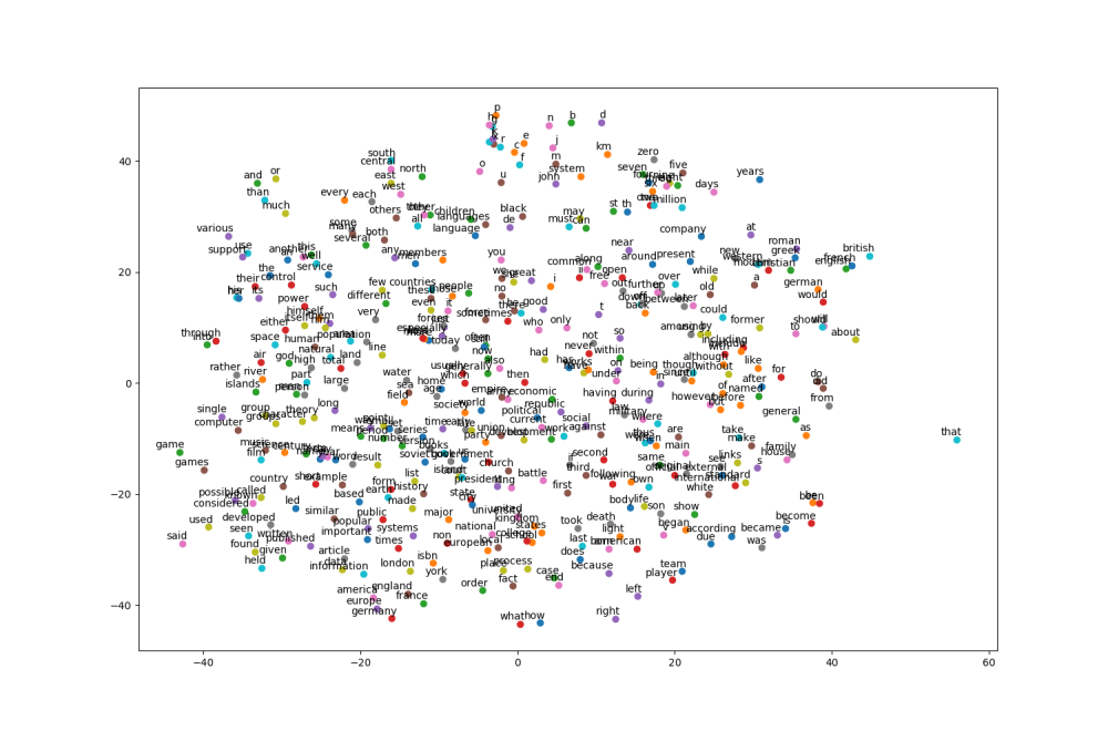
Skipgram

skipgram

CBOW

cbow

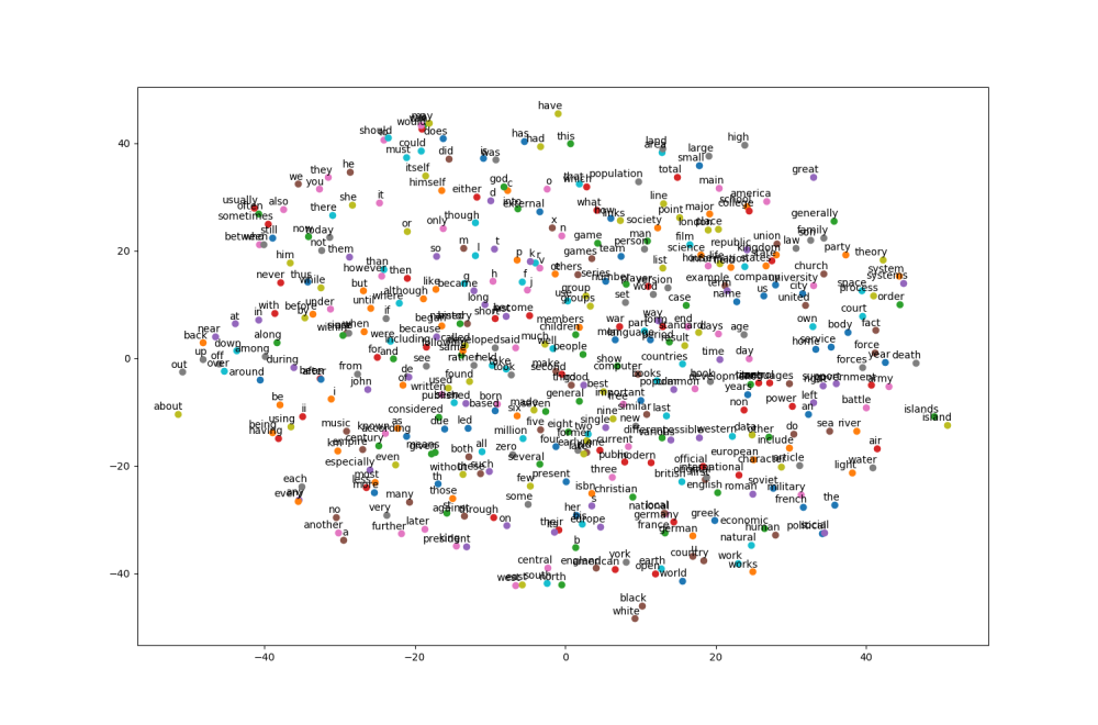
可以看出兩種作法都有出現群聚的結果，比如說英文字母在附近，數字在附近，介係詞在附近等等

再隨機從最常出現的字裡挑幾個來看看與其cosine distance最近的字們分別是什麼

Skipgram


Nearest to their: its, his, her, your, our, the, several, my
Nearest to that: which, what, however, who, golovachev, imperfect, but, eesti
Nearest to b: d, c, hafez, manager, katrina, ref, certificate, sage
Nearest to three: four, five, two, seven, eight, six, nine, zero
Nearest to called: named, used, referred, known, capua, vico, rouse, approximation
Nearest to with: between, weymouth, salicylate, at, including, agreeable, fright, in
Nearest to seven: eight, four, six, nine, five, three, zero, two
Nearest to such: well, known, including, certain, these, regarded, many, follows
Nearest to was: is, became, has, had, were, jn, been, valera
Nearest to have: had, has, are, include, having, were, require, contain
Nearest to often: sometimes, usually, generally, commonly, frequently, typically, now, still
Nearest to new: schema, salmonella, benedictine, monograph, crushes, separate, princely, weizenbaum
Nearest to war: pygmy, wars, connectionless, engaged, mitsuda, jerusalem, instincts, avril
Nearest to only: geopolitics, least, bitchx, fig, nance, stjepan, sceptical, rcs
Nearest to this: it, which, another, butterfield, the, he, there, some
Nearest to four: seven, five, six, eight, three, two, nine, zero

CBOW


Nearest to their: its, his, her, our, your, my, whose, discursive
Nearest to that: which, however, what, musicbrainz, cubism, emanation, kilmer, rosenberg
Nearest to b: d, te, cavalier, ares, twitching, blended, drank, sf
Nearest to three: five, four, six, seven, eight, two, nine, zero
Nearest to called: named, termed, considered, cited, jos, referred, known, used
Nearest to with: between, xiaoping, toward, rc, via, handguard, recapitulation, using
Nearest to seven: eight, five, four, six, nine, three, zero, two
Nearest to such: these, filesystems, certain, well, mentioned, geschichte, guderian, known
Nearest to was: is, became, were, had, has, lula, be, maintains
Nearest to have: had, has, are, were, include, having, feel, already
Nearest to often: usually, sometimes, frequently, commonly, typically, generally, normally, traditionally
Nearest to new: fourth, esteem, strange, third, fusion, ludlow, deanna, master
Nearest to war: buch, versailles, shrews, aas, apartheid, ruthenia, fao, passions
Nearest to only: substantially, especially, either, autumnal, telegram, talked, until, alternatively
Nearest to this: which, it, another, each, jacobitism, inquiries, what, the
Nearest to four: six, five, seven, three, eight, nine, zero, two

可以看出有些字做得不錯(像是seven, have等)，有些則是不理想(像是war, b, new等等)，再多跑幾次或是調整參數或是增加training set的大小應該都還能再更改善，不過這次就沒試了

還可以改進的地方

CBOW和Skip-Gram大體上相似只有在產生batch的方法不同以及graph有些微不同，或需應該讓兩個class都繼承自同一個class，只要改寫_generate_batch和_define_graph兩個方法即可
目前train的輸入只能接受一段文章，但在實際上使用應該是會送一大堆文章進去，在產生batch data及一開始train裡面將資料轉成array的地方需要做些修改

Vina Chang Blog

使用tensorflow實作word2vec CBOW

什麼是word2vec?

如何做word2vec?

CBOW與Skip-Gram的差異

CBOW(continuous bag of words)

Skip-Gram

共同參數:

graph的定義:

Skip-gram

generate_batch

CBOW

結果比較

Skipgram

CBOW

還可以改進的地方

發表留言取消回覆

什麼是word2vec?

如何做word2vec?

CBOW與Skip-Gram的差異

CBOW(continuous bag of words)

Skip-Gram

共同參數:

graph的定義:

Skip-gram

generate_batch

CBOW

結果比較

Skipgram

CBOW

還可以改進的地方

分享此文：

發表留言 取消回覆

發表留言取消回覆